Mutalisk can be used to investigate:
(1) Decomposition of mutational signatures
(2) Associations between various genome/epigenome regulatory elements
and somatic mutation rates across user-uploaded cancer genomes.
RUNNING THE DEMO
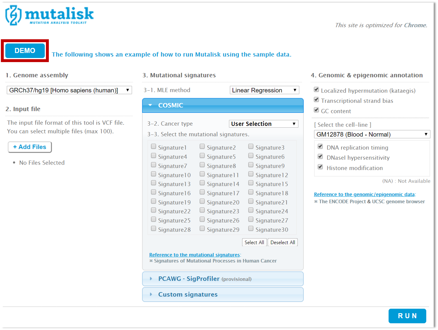
Step 1. Click on the Analyze tab

Step 2. Click on DEMO (top left)
Click on the DEMO button on the top left.
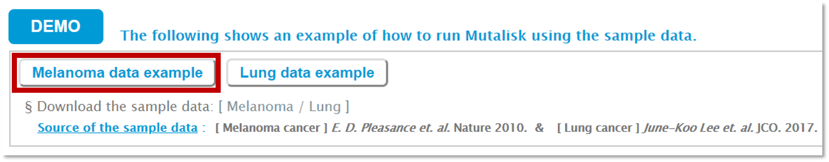
Step 3. Choose one of the sample caner genomes
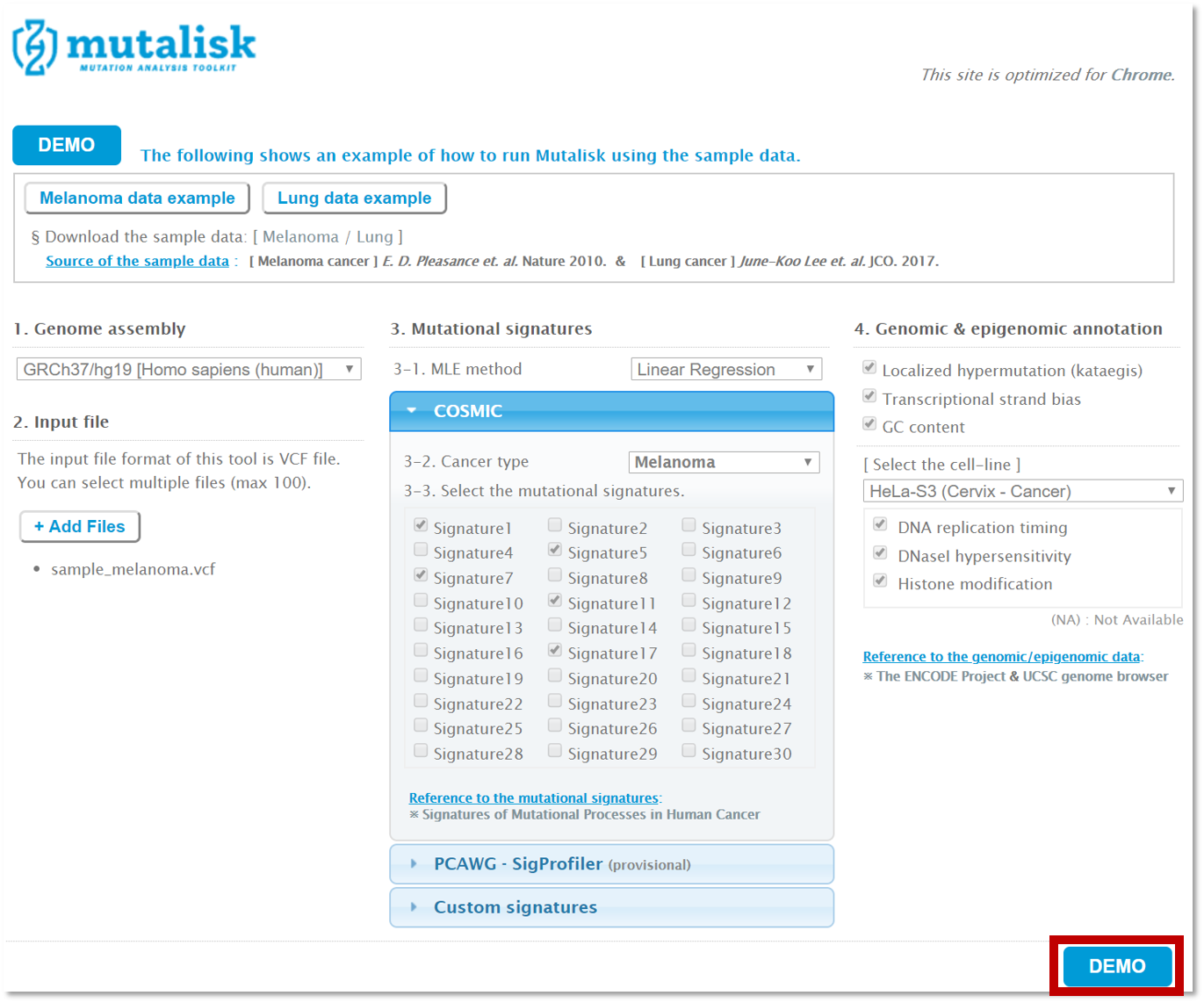
Click on either the melanoma or the lung cancer sample. You will notice that the analysis options for the mutational signatures and the genome assembly are automatically selected for the demo. You can also download the sample vcf files by clicking on the Melanoma or the Lung button.
Step 4. Click on DEMO (bottom right) to run the analysis
Click on the DEMO button on the bottom right.
RUNNING YOUR VCF FILE(S)
Step 1. Inputs/Options
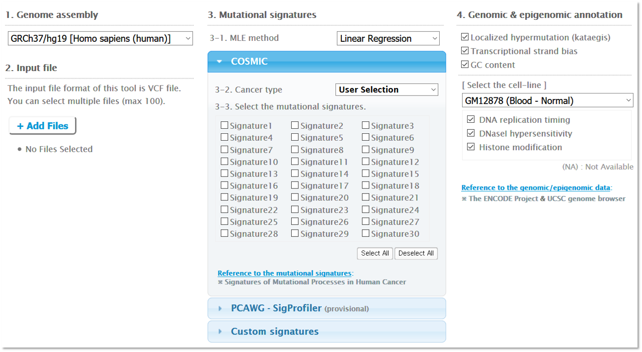
1. Genome assembly
Please specify the reference genome of the vcf files. Note that the reference genome must therefore be the same for all of the vcf files that you upload. Mutalisk currently supports hg19, hg38, and mm10. While we allow the decomposition of mutational signatures against the mouse genome assembly (mm10), the cancer mutational signatures are based on the human genome assembly; mm10 should be used at the user’s discretion.
2. Input file(s)
Each input file must be a vcf file. Each vcf file is decomposed and analyzed independently.
3. Mutational signatures
You can choose either the set of 30 COSMIC mutational signatures or the set of 65 PCAWG mutational signatures (SigProfiler). Alternatively, you may upload your own signature file.
3.1. Decomposition analysis method
Mutalisk models the decomposition of mutation signatures using the Maximum Likelihood Estimation (MLE) method. Two estimation methods are available: linear regression and multinomial test. A maximum of 7 mutational signatures are identified by Mutalisk as we conventionally expect 7 mutational signatures at most from a specific somatic tissue (Alexandrov et al., Cell 2013; Rahbari et al., Nature Genetics 2016; Serena et al., Nature 2016; Ju et al., Nature 2017; Polak et al., Nature Genetics 2017). Here we provide the source code used to run the decomposition analysis for your reference. The sub-sections (3.1.1-3) below describe how Mutalisk performs the analysis for each suite of mutational signatures. [ Source Code Download ]
3.1.1. COSMIC
For the decomposition analysis using the 30 COSMIC signatures, Mutalisk employs a greedy algorithm to identify relevant mutational signatures underlying the observed mutational profile. From the user-specified selection of n signatures, Mutalisk traverses through the search space of up to 7-combinations (k = 1…7; n choose k) without repetition while only choosing the next best signature in subsequent k-combination. For each set of k-signatures, a decomposition model is generated by the Maximum Likelihood Estimation (MLE) method using the optim function in R while minimizing a constrained function either by a linear function or by -2 x natural logarithm of likelihood ratio (multinomial test). At each k-combination, Mutalisk identifies the best combination of k-signatures based on the value parameter returned from the optim function. In the subsequent combination, k+1, Mutalisk only considers combination elements that include the set of signatures chosen up to k-combinations. It should be noted that Mutalisk chooses the first signature as part of the best decomposition model after exploring up to 3-combinations (k = 1…3). This is a heuristic that we implemented to prevent early local optimization bias. As a result, Mutalisk identifies up to 7 best decomposition models and ranks these based on Bayesian information criterion (BIC) to discourage overfitting.
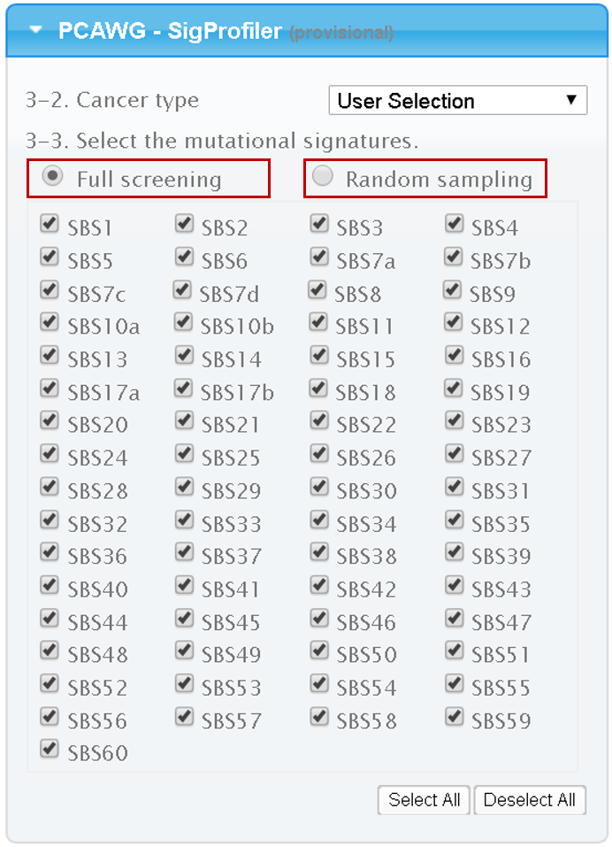
3.1.2. PCAWG
If 30 or fewer PCAWG signatures are selected, then Mutalisk employs the same greedy method used for the COSMIC signatures. However, if more than 30 signatures are selected, the user is presented with two options to run the analysis: the aforementioned greedy algorithm described above ("Full screening") and another approach that combines the greedy approach with a series of hill climbing with randomly selected signatures ("Random sampling"). The random sampling method generates results relatively faster but the resulting selection of signatures with smaller contribution probabilities can be different between two independent analysis runs due to the random generation of initial states. In this approach, Mutalisk randomly selects 20 signatures by sampling without replacement and then performs the aforementioned greedy algorithm on the 20 signatures to find locally optimal 7 signatures. This process is repeated 20 times, generating 20 sets of 7 signatures. Finally, Mutalisk applies the greedy algorithm using the signatures (contribution probability > 0.05) identified in these 20 sets.
3.1.3. Custom Signatures
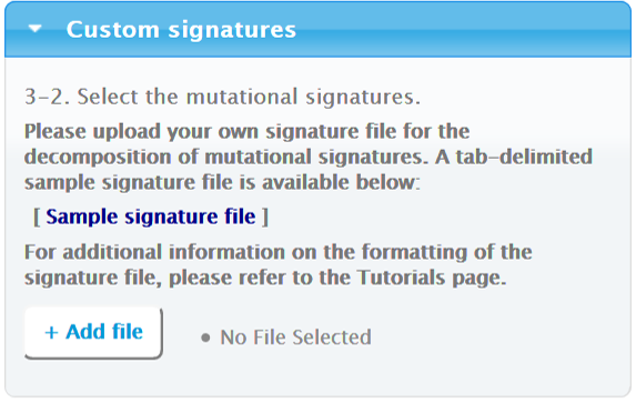
If you choose to perform the mutational signature decomposition using your own signatures, Mutalisk uses the greedy approach described above. Mutalisk uses up to the first 30 signatures in the tab-delimited file to perform the analysis.
Please note that the file must be tab-delimited with the following format:

You may also refer to the sample signature file (.txt) downloadable from the Custom signatures tab.
3.2. Cancer type
You can select mutation signatures either by selecting a preset cancer type or by manually selecting each signature of your interest. Selection of multiple signatures is possible. Please note that if you select one of the first 7 options (Hematologic Malignancy, Alimentary Tract, Brain Cancer (adult), Brain Cancer (pediatric), Kidney Cancer, Lung Cancer, or Uterus Cancer) under “Cancer type”, the signatures from each subtype will be combined together. For example, “Lung Cancer” is the combination of all signatures present in Lung Adeno, Lung Small Cell, and Lung Squamous.
4. Genomic and epigenomic annotation
Select the genomic/epigenomic annotations that you wish to perform: localized hypermutation (kataegis), transcriptional strand bias analysis, or GC-content analysis. Also, select which reference cell line genome and epigenome data will be used to analyze the associations between each regulatory element and the somatic mutation rates.
Step 2. Running the analysis
Once you have finished specifying the configurations, click on the RUN button on the bottom right.
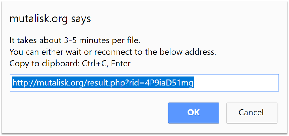
✔ Link to results
You will see a popup window on the screen. The analysis computation time depends on the input file size. For your convenience a link is provided to the results page so that the analysis outputs can be viewed later. Results are stored on Mutalisk for 48 hours, after which the results data are permanently deleted. For your information, the sample lung cancer (hg19) vcf file along with the lung cancer COSMIC signatures and the multinomial test option may take around 5 minutes to process.
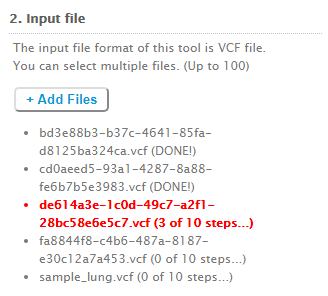
✔ Progress status
For each vcf file that you upload, we keep you informed on the progress of the analysis computation.
INTERPRETING RESULTS
1. Localized hypermutation
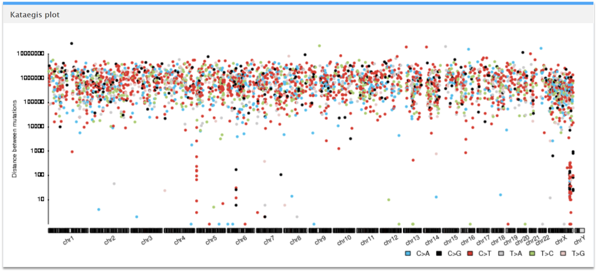
This rainfall plot of the sample lung cancer mutations shows the distances between the mutations and can be used to infer whether localized hypermutations (kataegis) exist in this vcf file. The dots represent the mutations and the different colors represent each of the 6 subtypes of base substitutions: C>A, C>G, C>T, T>A, T>C, and T>G. Here, we observe kataegis in chromosomes 5, 6 and X.
2. Mutational signatures
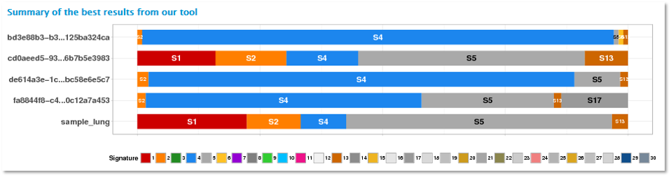
The graph above shows the best mutational signature decomposition model for each vcf file.
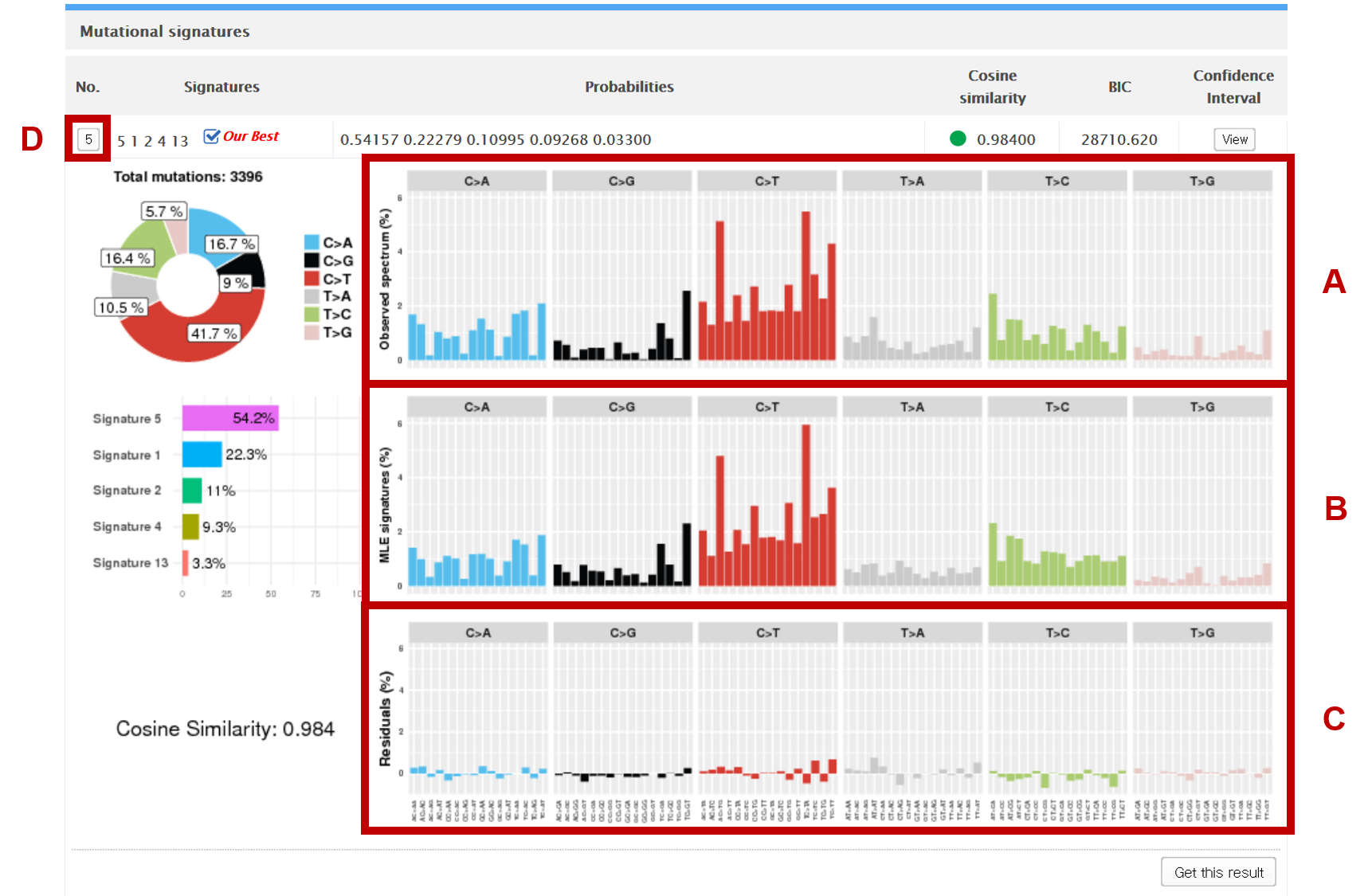
The pie chart on the top left shows the percentage of each subtype found in the vcf file. A (see the figure above) shows the observed distribution of mutations across the 96 possible mutation types (6 types of substitution * 4 types of 5’ base * 4 types of 3’ base). B shows the summation of the distributions of the decomposed signatures. C shows the difference of each base substitution subtype between A and B.
Clicking on “Get this result” on bottom right downloads a zipped folder of the model parameters and metadata.
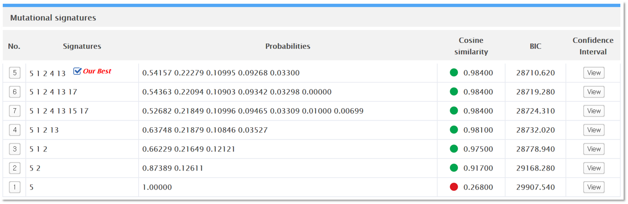
Index (No.)
The index number specifies the number of decomposed signatures in each model. Clicking on D collapses the model view and presents a table (see the figure below) of up to 7 best decomposition models generated by Mutalisk. The best of the 7 models is indicated with the label “Our Best”, based on the ranking by Bayesian information criterion (BIC). If you click on each index number, you can see a more detailed view of the specific model. You can expand multiple indices to visually compare different decomposition models.
Signatures
The “Signatures” column lists the mutation signatures identified in each model.
Probabilities
Each probability denotes the probability of observing the given signature; the order of probabilities corresponds to the order found in the “Signatures” column.
Cosine similarity
Cosine similarity is computed between the distribution of mutations in the vcf file and the set of signatures identified in the “Signatures” column.
BIC
BIC refers to the Bayesian information criterion score computed for each model. BIC score was used to rank the models (in ascending order).
Confidence interval
Click on “View” to see the 95% confidence interval for each probability in the “Probabilities” column.
3. Transcriptional strand bias
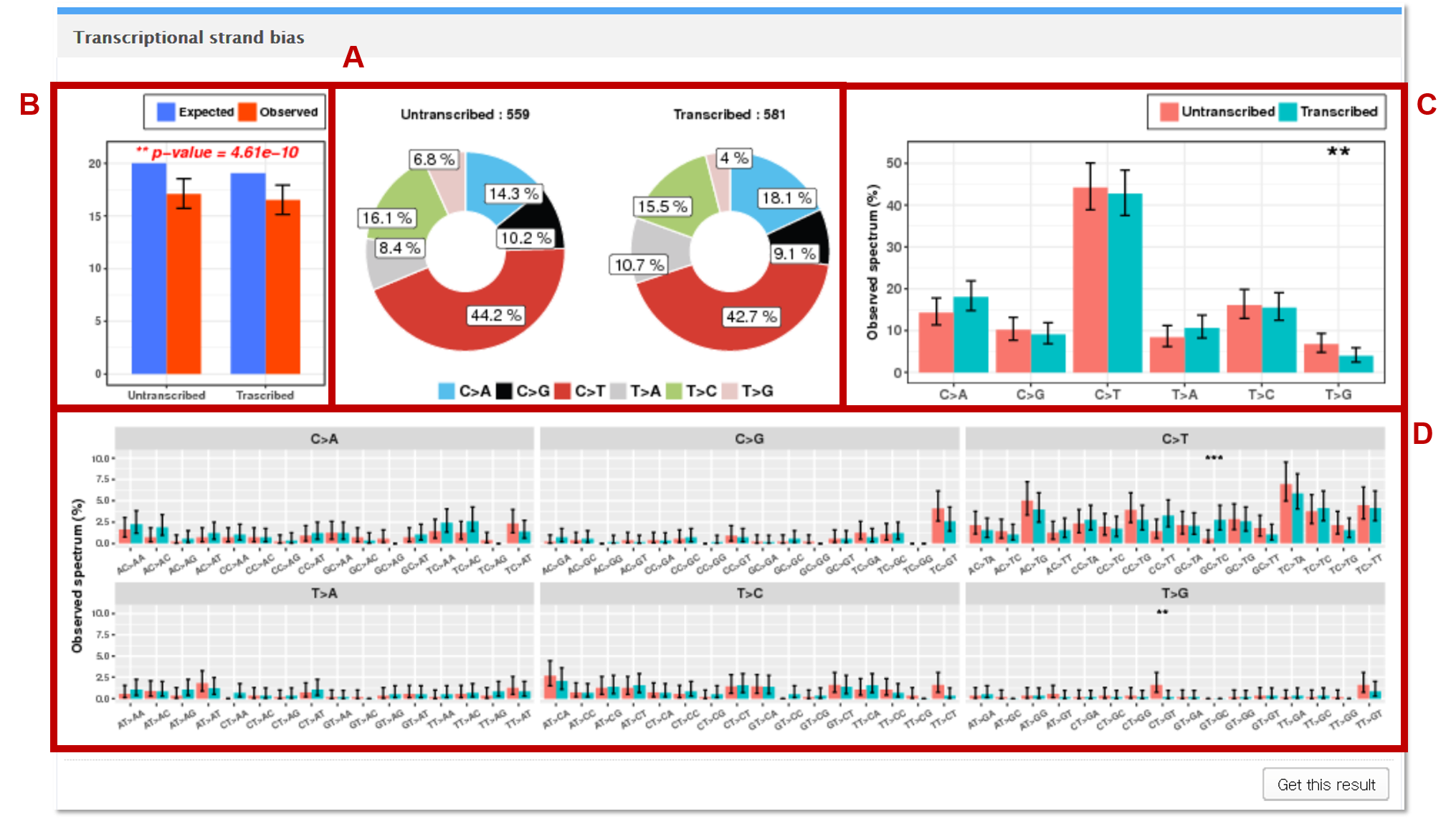
Mutalisk identifies mutations in the vcf file that map to the coding region of the selected genome assembly. The transcription direction (forward or reverse) of the mapped genes are annotated. The mutations are then categorized into one of the 6 base substitution subtypes. If the representative base substitution (C>A, C>G, C>T, T>A, T>C, and T>G) is on a forward strand gene, then Mutalisk defines the mutation to be in an untranscribed region, and in a transcribed region if the representative substitution is on a reverse strand gene.
In the example below, we see that there are 787 mutations in the untranscribed mutations and 854 transcribed mutations, and 1755 mutations do not map to any genes (3396 - 787 - 854 = 1755).
A The observed counts of mutation for each of the 6 base substitution subtypes in untranscribed and transcribed regions are presented as pie charts.
BGoodness of fit test (chi-square test) is performed to test whether the observed mutations counts from transcribed and untranscribed regions are significantly different from the expected proportions of the untranscribed and transcribed regions in the selected genome assembly (**, *** = p-value < 0.05 and 0.01 respectively).
CEach statistical significance indicates whether the mutation counts for untranscribed and transcribed regions for the specific base substitution subtype (e.g. C>A) are significantly different from the mutations counts for untranscribed and transcribed regions in the other 5 subtypes.
DEach independence test for all 96 possible mutation types (6 subtypes of base substitution * 4 types of 5’ base * 4 types of 3’ base) is computed between the mutation counts for untranscribed and transcribed regions for the specific combination (AC>TA) of the given base substitution subtype (e.g. C>T) and the other 15 combinations of the same base substitution subtype.
4. Correlation and percentage of explained variance
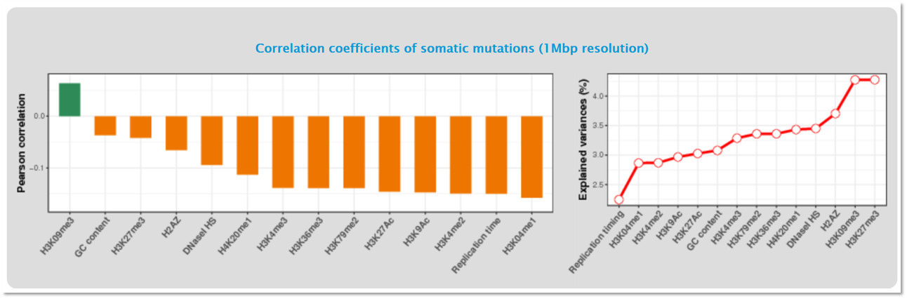
Mutalisk calculates the Pearson correlation between the read density of each regulatory element and the mutation frequencies at 1-megabase (Mb) intervals. The graph on the left shows the correlation coefficient values for each regulatory element. The graph on the right shows how much of the features can explain the mutation rate across the cancer genome at 1-Mb.
5. GC-content
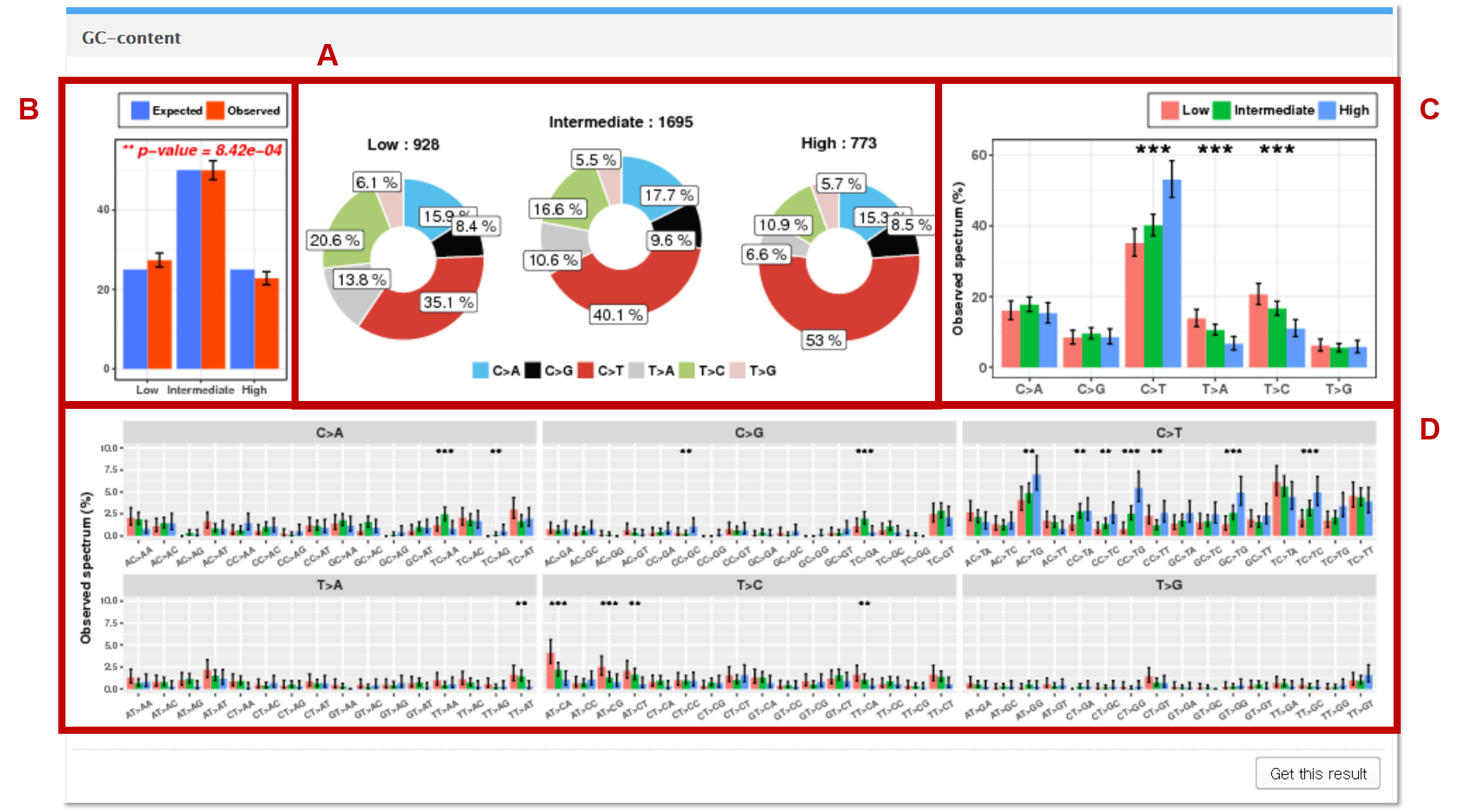
The mutations in the vcf file are mapped to the genomic regions (1,000bp windows) of low, intermediate, and high GC-contents.
AThe observed counts of mutation for each of the 6 base substitution subtypes in low, intermediate, and high GC-content regions are presented as pie charts.
BGoodness of fit test is performed to test whether the observed mutation counts in genomic positions corresponding to low, intermediate, and high GC-content are significantly different from the expected proportions of the selected genome assembly.
CEach statistical significance indicates whether the mutation counts for low, intermediate, and high GC-content regions for the specific base substitution subtype (e.g. C>A) are significantly different from the mutations counts for low, intermediate, and high GC-content regions in the other 5 subtypes.
DEach independence test for all 96 possible mutation types (6 subtypes of base substitution * 4 types of 5’ base * 4 types of 3’ base) is computed between the mutation counts for low, intermediate, and high GC-content regions for the specific combination (AC>TA) of the given base substitution subtype (e.g. C>T) and the other 15 combinations of the same base substitution subtype.
6. DNA replication timing
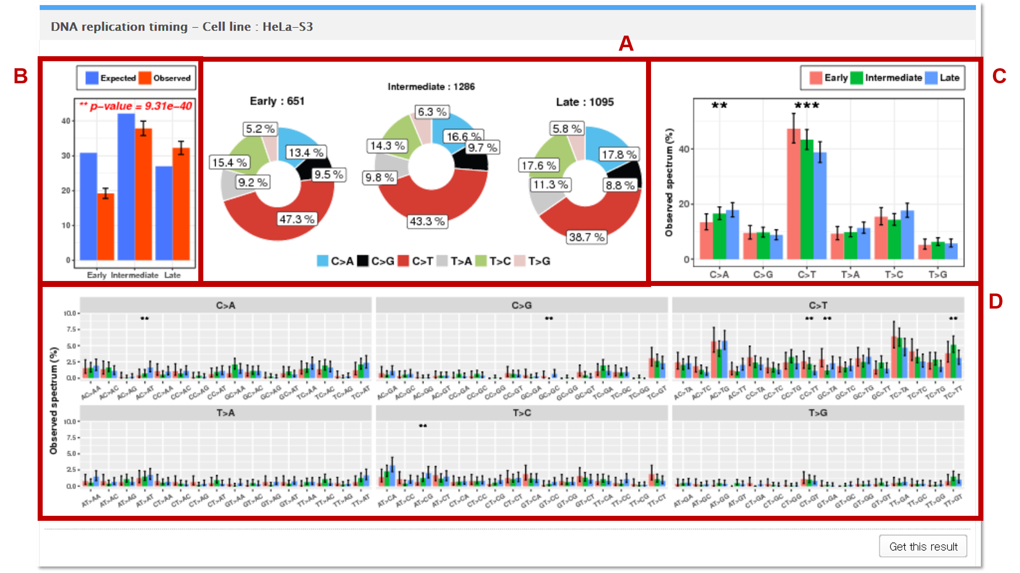
The mutations in the vcf file are mapped to the genomic regions (1,000 bp windows) of early (G1, S1), intermediate (S2, S3), and late (S4, G2) replication timing phases. The Repli-seq data were obtained from ENCODE to achieve this task. Note that there are genomic regions that do not map one of the three phases, and mutations that map to these regions are classified as unknown. In the example above, 364 mutations (3396 - 651 - 1286 - 1095 = 364) map to the unknown regions.
AThe observed counts of mutation for each of the 6 base substitution subtypes in early, intermediate, and late phase regions are presented as pie charts.
BGoodness of fit test is performed to test whether the observed mutation counts in genomic positions corresponding to early, intermediate, and late phases are significantly different from the expected proportions of the selected genome assembly.
CEach statistical significance indicates whether the mutation counts for early, intermediate, and late phase regions for the specific base substitution subtype (e.g. C>A) are significantly different from the mutations counts for untranscribed and transcribed regions in the other 5 subtypes.
DEach independence test for all 96 possible mutation types (6 subtypes of base substitution * 4 types of 5’ base * 4 types of 3’ base) is computed between the mutation counts for early, intermediate, and late phase regions for the specific combination (AC>TA) of the given base substitution subtype (e.g. C>T) and the other 15 combinations of the same base substitution subtype.
7. DNase I hypersensitivity
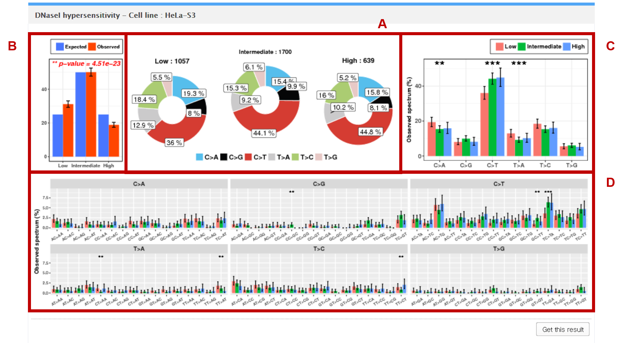
The mutations in the vcf file are mapped to the genomic regions (1Mbp windows) of low, intermediate, and high peaks of DNase I hypersensitivity. DNase I hypersensitivity data were obtained from the ENCODE project.
AThe observed counts of mutation for each of the 6 base substitution subtypes in low, intermediate, and high peak regions are presented as pie charts.
BGoodness of fit test is performed to test whether the observed mutation counts in genomic positions corresponding to low, intermediate, and high peaks are significantly different from the expected proportions of the selected genome assembly.
CEach statistical significance indicates whether the mutation counts for low, intermediate, and high peak regions for the specific base substitution subtype (e.g. C>A) are significantly different from the mutations counts for low, intermediate, and high peak regions in the other 5 subtypes.
DEach independence test for all 96 possible mutation types (6 subtypes of base substitution * 4 types of 5’ base * 4 types of 3’ base) is computed between the mutation counts for low, intermediate, and high peak regions for the specific combination (AC>TA) of the given base substitution subtype (e.g. C>T) and the other 15 combinations of the same base substitution subtype.
8. Histone modifications
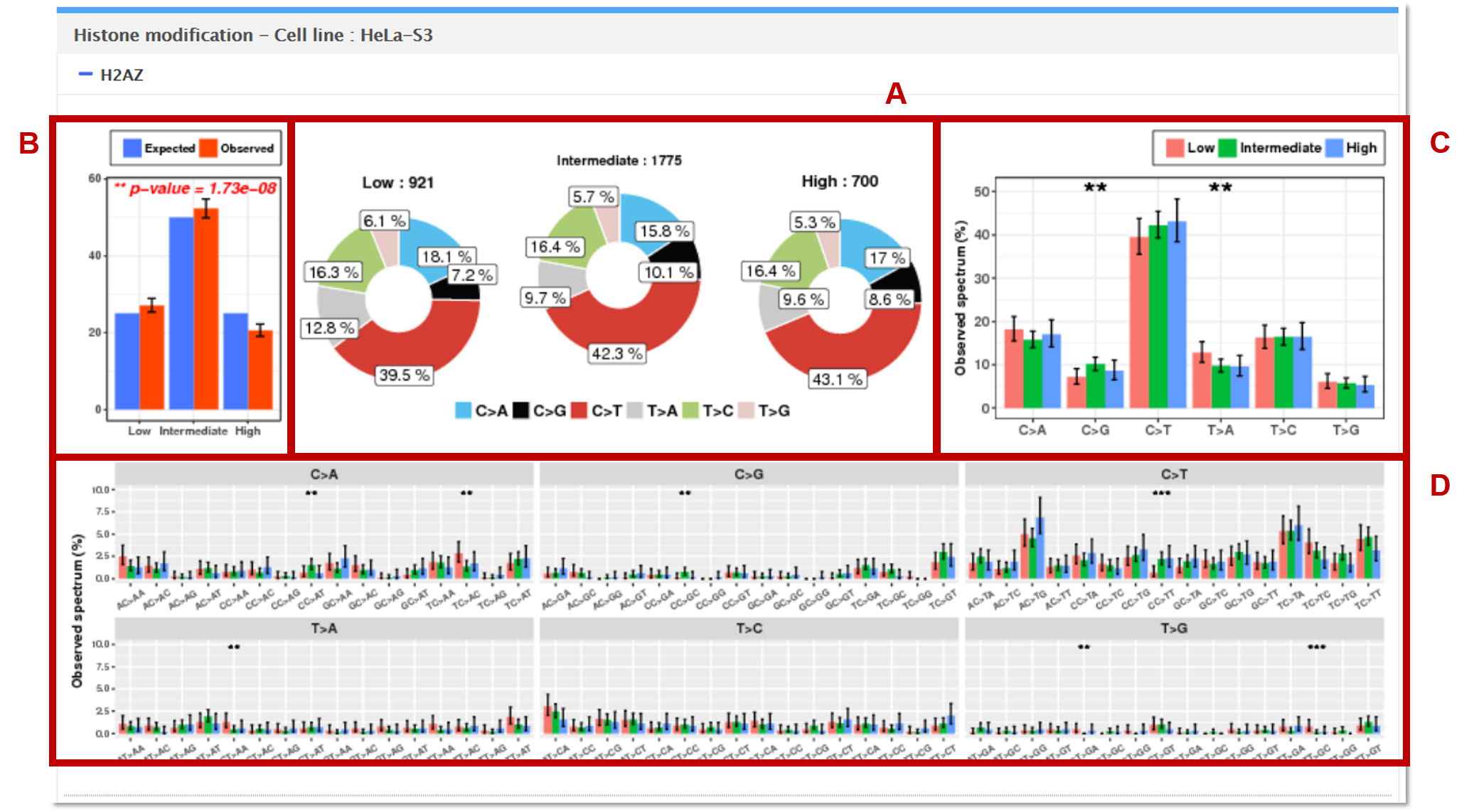
The mutations in the vcf file are mapped to the genomic regions (1Mbp windows) of low, intermediate, and high peaks from ChIP-seq for each histone modification. Histone modification data were obtained from the ENCODE project. Mutalisk analyzes each histone modification separately.
AThe observed counts of mutation for each of the 6 base substitution subtypes in low, intermediate, and high peak regions are presented as pie charts.
BGoodness of fit test is performed to test whether the observed mutation counts in genomic positions corresponding to low, intermediate, and high peaks are significantly different from the expected proportions of the selected genome assembly.
CEach statistical significance indicates whether the mutation counts for low, intermediate, and high peak regions for the specific base substitution subtype (e.g. C>A) are significantly different from the mutations counts for low, intermediate, and high peak regions in the other 5 subtypes.
DEach independence test for all 96 possible mutation types (6 subtypes of base substitution * 4 types of 5’ base * 4 types of 3’ base) is computed between the mutation counts for low, intermediate, and high peak regions for the specific combination (AC>TA) of the given base substitution subtype (e.g. C>T) and the other 15 combinations of the same base substitution subtype.
DOWNLOADING RESULTS
You can either (A) download all of the analysis results merged into one text file or (B) download a zipped file of each analysis results saved into an individual text file. Alternatively, you may click on the “Get this result” button under each analysis. This downloads a zipped file of the corresponding analysis results only.

1. Mutational signatures
The unzipped folder consists of 2 files for each vcf file that the user uploaded:
vcf_file_name_cancer_type_report.pdf
vcf_file_name_cancer_type_report.txt
The .txt file contains the following data (based on the sample.vcf file):
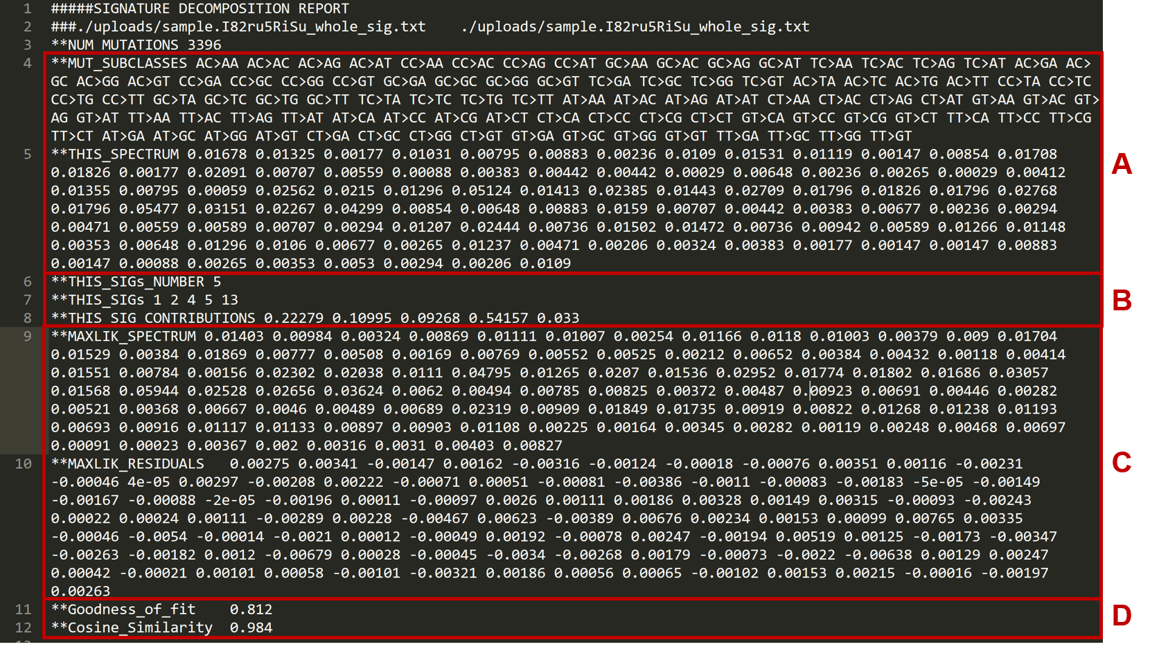
ALines 5 is the spectrum of each of the 96 possible mutations types, specified by line 4.
BLines 6 to 8 include the data on Mutalisk’s best decomposition model of mutational signatures. Line 6 indicates the total number of signatures included in the best decomposition. Here we see that the signatures 1, 2, 4, 5, and 13 (line 7) each contribute 0.22279, 0.10995, 0.09268, 0.54157, and 0.033, respectively (line 8), to the decomposition.
CLine 9 specifies the estimated spectrum of each of the 96 mutation types from the best decomposition. Line 10 is the residual between the actual spectrum (line 5) and the estimated spectrum (line 9).
DThe goodness of fit and cosine similarity scores of the best decomposition model.
2. Transcriptional strand bias, DNA replication timing, GC-content, histone modification
The unzipped folder consists of 1 pdf file and 2 or 3 vcf files for each category of the sub-analysis. Each vcf file contains mutations mapped to each category of the sub-analysis.